Gravitational lensing

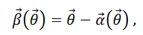
To calculate the position, shape and size of the image from a specific source we use the so called lens equation:

where α is the reduced deflection angle of the light rays. The interpretation of the lens equation is that a source with true position β can be seen by an observer at angular positions θ satisfying the lens equation. If the equation has more than one solution for fixed β, that source has images at several positions on the sky, i.e. the lens produces multiple images.

In this simulation we only examine cases in which the lens has circular symmetry, so we don't need the vectors, only the modulus of them.

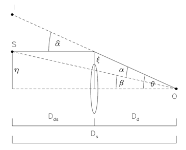
Sketch of a typical gravitational lens system

The deflection angle and the deflection potential of the lens are related by

The distortion of images is described by the Jacobian matrix that tells us how β changes when θ is manipulated, that is

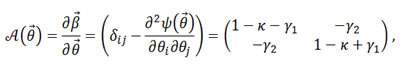
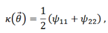
where we have defined the convergence

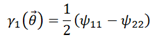
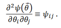
and the shear components

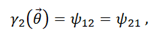
and

with the abbreviation

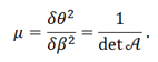
The ratio of the image and source flux is the magnification μ. A solid-angle element of the source δβ² is mapped to the solid-angle element of the image δθ²; so the magnification is

Points in the lens plane where detA=0 form closed curves, called critical curves. Their corresponding curves in the source plane are the caustics. So if we know the deflection potential of the lens we can calculate κ, γ₁ and γ₂, and with those we can obtain the θ-s that satisfy detA=0, that is, the critical curves. Using the lens equation we can calculate the corresponding β-s, the caustics. Critical lines and caustics are important because they highlight regions of high magnification and they demarcate regions of different image multiplicity. When the source is out of all caustics we will see a single image. Each time it crosses a caustic the image number changes by +2.